Examples

Example 1: Log-Normal

To sample from the log-normal distribution:

import numpy as np
import scipy
from rusampling import Ru

logf = scipy.stats.lognorm.logpdf

t = Ru(logf, s=1)
samples = t.rvs(n=100000)
t.plot()

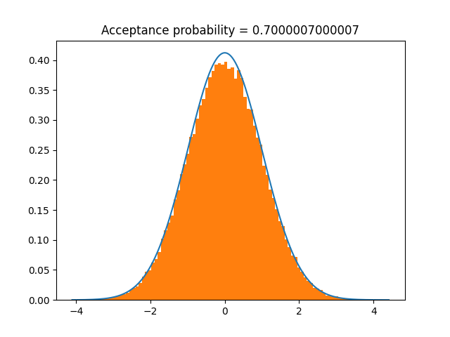
Or, we can use \(X=\log(x)\) to transform to a normal distribution, sample from that, and transform back. This improves the acceptance probability, so samples faster.

We have to pass the inverse transform, \(x(X) = e^X\), and the log-Jacobian of this transform, which is \(X\).

I have set undo_transformations=False in rvs for illustrative purposes.

import numpy as np
import scipy
from rusampling import Ru

logf = scipy.stats.lognorm.logpdf

t = Ru(
    logf, s=1,
    X_to_x = lambda X: np.exp(X), 
    X_to_x_logj = lambda X: X
)
samples = t.rvs(n=100000, undo_transformations=False)
t.plot()

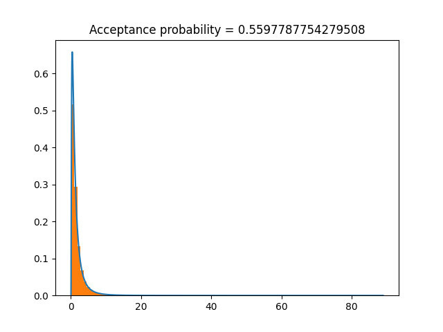
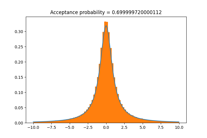
Example 2: Cauchy Distribution

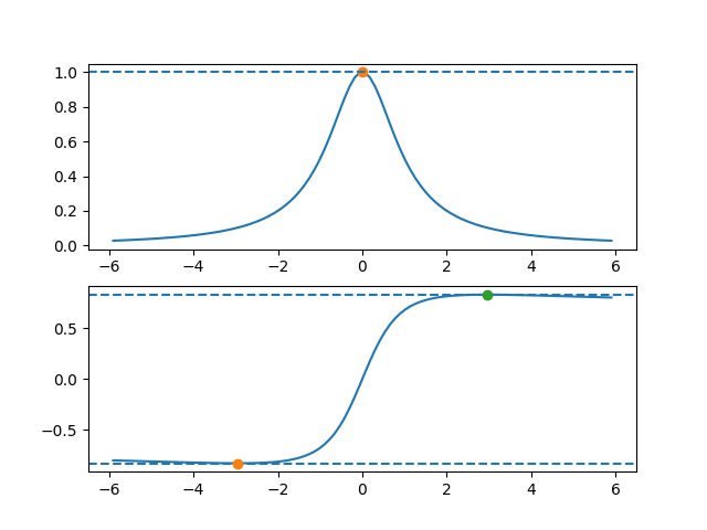
The bounding box for the Cauchy distribution does not exist if r < 1. For values > 1, r=1.26 gives the optimal acceptance probability. I used the plot_f method to check the bounding box is in the right place.

import scipy.stats as stats
from rusampling import Ru

t = Ru(stats.cauchy.logpdf, r=1.26)
t.plot_f()                              # check that the rectangle is found correctly
t.rvs(n=500000)
t.plot(bins=80, xmax=10, xmin=-10)     # plot a histogram of results

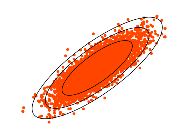
Example 3: Gamma Distribution Parameter Sampling

Generate samples from the gamma distribution, then sample the shape and scale. The prior is \(\frac{1}{a \sigma }\), chosen for reliability (see our paper on this topic).

Note that in order to sample quickly, the logpdf must be vectorised in whichever variable is to be sampled. SciPy does not provide logpdfs that are vectorised in the parameters, so this is done by hand.

import numpy as np
import scipy.stats
from rusampling import Ru

def gamma_logf(params, x):                                  # Posterior distribution for gamma
    m = np.maximum(params, np.finfo(np.float64).eps)
    sh, sc = m[:,0], m[:,1]                                 # shape, scale
    x_scaled = x[:,None]/sc
    
    g = scipy.special.gamma(sh)                             # Computing components of the gamma logpdf
    x_sum = np.sum(x_scaled, axis=0)
    log_x_sum = np.sum(np.log(x_scaled), axis=0) 
    log_pdf = -len(x)*np.log(g*sc) + (sh-1)*log_x_sum - x_sum
    log_prior = - np.log(sh) - np.log(sc)
    return log_pdf + log_prior


data = scipy.stats.gamma.rvs(a=0.5, scale=5, size=200)      # Generate training data from the gamma distribution

t = Ru(gamma_logf, x=data, d=2)        
t.plot_f(                                                   # Confirm that the bounding rectangle is correct with contour plots
    levels = 20,
    n_points = 100, 
    xlim=np.asarray(((-0.5, 0.5), (-1, 1), (-0.75, 0.75))), 
    ylim=np.asarray(((-0.5, 0.5), (-1, 1), (-0.5, 0.8))),
    )
y = t.rvs(n=10000) 
t.plot(s=1, color='orangered')

The output from plot_f, below, has crosses at the maxima and minima:

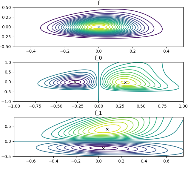
And the output from plot:

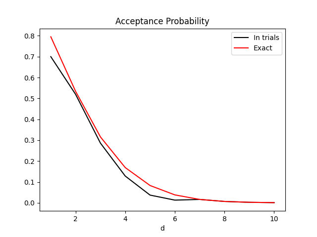
Example 4: Acceptance Probability drop-off

Wakefield, Gelfand, and Smith (1991) present a formula for acceptance probability in Efficient generation of random variates via the ratio-of-uniforms method. Application to the n-dimensional Gaussian gives the expression $$P_a = \frac{(\pi/2)^\frac d2}{(1+rd)(\frac{1+rd}{er})^\frac d2}$$ I plotted this expression against d, together with the actual acceptance rate over 100,000 trials, in order to visualise the insuitability of Ratio-of-Uniforms in high dimensions.

This example makes use of the option to provide the derivative of logf for a more accurate bounding rectangle in higher dimensions.

Open code in new tab.