Details

t refers to an instance of the Ru class.

Init

Parameters when initialising t:

• logf

  Should accept a shape (n, d) np.array and return a shape (n,) np.array. In the d=1 case, acceps x as either (n, 1) or (n,).

  Non-vectorised functions are also supported, i.e. (d,) -> float (or d=1: float -> float). However, if possible, vectorise your function over multiple x values using numpy broadcasting, as this massively speeds up the sampling.

• **logf_args

  Extra keyword arguments that logf takes.

• d=1

  Dimension of the random variable.

• ics = [0, .., 0]

  Initial conditions with which to find the mode of f. A d-dimensional list.

  If Ru fails, check these first; in particular, make sure they lie in a region where f is not identically zero.

• X_to_x = None, X_to_x_logj = None

  User-defined transformation to apply (first) to the space. (The transformation is undone before samples are returned.)

  If, say, the transformation is X(x), the inverse x(X), i.e. 'X-to-x', must be passed, as well as the log-Jacobian of this inverse.

  It is assumed that initial conditions passed have had this transformation applied, so are values of X, not x.

• YJ_lambda = None

  The Yeo-Johnson transformation is applied if lambda are supplied as a d-dimensional list. This may increase acceptance probability.

• logf_jac = None

  Function (n,) -> (n,) (n-dim array to n-dim array). Derivative of logf. Provide if using an optimisation algorithm that requires it.

• optim_method_mode = 'Nelder-Mead'

  Method used to find the mode of logf.

  Methods that use the derivative, e.g. BFGS, usually perform better, if you have the derivative of logf to hand. See the SciPy docs on scipy.optimize.minimize for methods.

• optim_method_auxiliary = 'Nelder-Mead'

  Method used to find the inf/sup of auxiliary functions \(x_i f^ \frac{r}{1+rd}\). See above.

• r = 0.5

  Tuning parameter to use in the Ratio-of-Uniforms algorithm, which affects the acceptance probability. r=0.5 is optimal in the Gaussian case.

• rotate = True

  Reducing the correlation between the dimensions of the random variable can improve acceptance probability. Ru attempts to do this by rotating the axes. Applies when d>1.

• rectangle = None

  The bounding rectangle for f is calculated automatically. If you wish to calculate it separately, provide a (2, d)-dimensional numpy array, where (0, :) are the minimums and (1, :) the maximums.

Sampling

After initialising, call:

• t.rvs(n=N) to return a (N, d) numpy array of samples.
• t.rvs_detail(n=N) (instead of rvs) to return a dict with keys 'rvs' (samples), 'pa' (acceptance probability) and 'time' (elapsed during sampling).
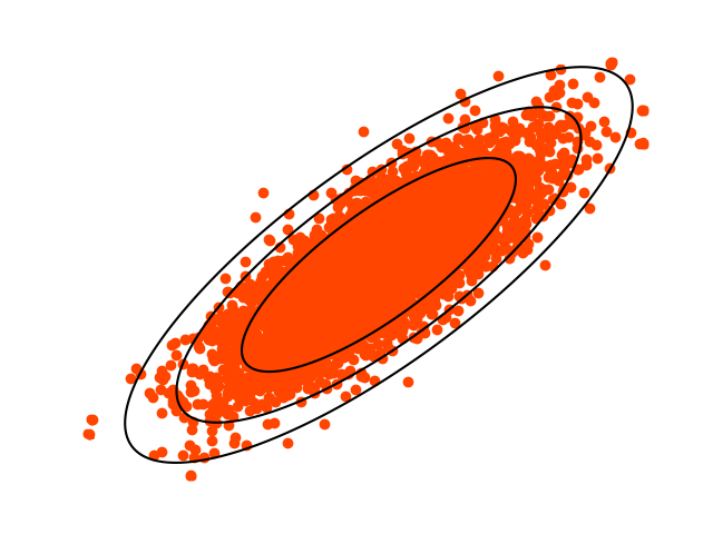
• t.plot() for d=1,2, after generating samples to plot the samples in a histogram/scatter plot against f.
• t.f() for the transformed function which the algorithm is applied to; t.f_original() is the original pdf.
• t.info() to print out the bounding rectangle.
• t.plot_f() for d=1, 2 to confirm that the bounding rectangle has been found correctly.
• Pass undo_transformations=False to either rvs or rvs_detail of these to return the transformed variable.